Outputs of DeepPrep

The outputs of DeepPrep have three categories:

Anatomical derivatives: The anatomical images are preprocessed through motion correction, tissue segmentation, cortical surface reconstruction, volume and cortical surface registration, and etc.
Functional derivatives: The functional images are preprocessed through motion correction, slice timing correction, susceptibility distortion correction, confounds estimation, and registration to both standard and non-standard spaces.
Visual reports: For better visualization and understanding of the entire process, DeepPrep generates a visual report for each subject.

Anatomical derivatives

FreeSurfer carries out preprocessed anatomical derivatives store in <output_dir>/Recon by default:

<output_dir>/
├── Recon/
├── fsaverage/
├── sub-<subject_label>/
├── sub-<subject_label>/
    ├── label/
    ├── mri/
    ├── scripts/
    └── ...
└── ...

The preprocessed structural MRI data are organized to align with the results of FreeSurfer, encompassing the normalized and skull-stripped brain, reconstructed cortical surfaces and morphometrics, volumetric segmentation, cortical surface parcellation, and their corresponding statistics. Additionally, transformation files for surface spherical registration are included.

Functional derivatives

The preprocessed functional derivatives are stored under the <output_dir>/BOLD in BIDS structure. All entities are shown in the file names, where sub-<subject_label> is mandatory, and the rest are optional:

<output_dir>/
├── BOLD/
├── sub-<subject_label>/
├── sub-<subject_label>/
    ├── anat/
        ├── sub-<subject_label>_space-<space_label>_res-<resolution>_desc-noskull_T1w.nii.gz
        ├── sub-<subject_label>_space-<space_label>_res-<resolution>_desc-noskull_T1w.nii.gz
        └── ...
    ├── figures/
        ├── sub-<subject_label>_task-<task_label>_run-<run_idx>_desc-summary_bold.html
        └── ...
    └── func/
        ├── sub-<subject_label>_task-<task_label>_run-<run_idx>_from-orig_to-boldref_mode-image_desc-hmc_xfm.txt
        ├── sub-<subject_label>_task-<task_label>_run-<run_idx>_space-<space_label>_res-<resolution>_desc-preproc_bold.nii.gz
        └── ...
├── ...
└── dataset_description.json

The default output spaces for the preprocessed functional MRI consist of three options: 1. the native BOLD fMRI space, 2. the MNI152NLin6Asym space, and 3. the fsaverage6 surfaces space. However, users have the flexibility to specify other output spaces, including the native T1w space and various volumetric and surface templates available on TemplateFlow. The main outputs of the preprocessed data include:

1.Preprocessed fMRI data.

2.Reference volume for motion correction.

3.Brain masks in the BOLD native space, include the nuisance masks, such as the ventricle and white-matter masks.

4.Transformation files for between T1w and the fMRI reference and between T1w and the standard templates.

5.Head motion parameters and the temporal SNR map.

6.Confound matrix.

Preprocessed fMRI data are stored in the <output_dir>/func and <output_dir>/anat along with their reference files and json files:

sub-<subject_label>/
├── anat/
    ├── sub-<subject_label>_desc-brain_mask.nii.gz
    ├── sub-<subject_label>_desc-preproc_T1w.nii.gz
├── func/
    ├── sub-<subject_label>_task-<task_label>_run-<run_idx>_space-<space_label>_res-<resolution>_desc-preproc_bold.nii.gz
    ├── sub-<subject_label>_task-<task_label>_run-<run_idx>_space-<space_label>_res-<resolution>_desc-preproc_bold.json
    ├── sub-<subject_label>_task-<task_label>_run-<run_idx>_space-<space_label>_desc-brain_mask.nii.gz
    ├── sub-<subject_label>_task-<task_label>_run-<run_idx>_space-<space_label>_res-<resolution>_desc-preproc_boldref.nii.gz

Motion correction outputs include motion corrected BOLD, reference frame to align with, and transformation matrices:

sub-<subject_label>/
├── func/
    ├── sub-<subject_label>_task-<task_label>_run-<run_idx>_desc-hmc_boldref.nii.gz
    ├── sub-<subject_label>_task-<task_label>_run-<run_idx>_desc-hmc_boldref.json
    ├── sub-<subject_label>_task-<task_label>_run-<run_idx>_bold_mcf.nii.gz_abs.rms
    ├── sub-<subject_label>_task-<task_label>_run-<run_idx>_bold_mcf.nii.gz_rel.rms
    ├── sub-<subject_label>_task-<task_label>_run-<run_idx>_bold_mcf.nii.gz.par
    ├── sub-<subject_label>_task-<task_label>_run-<run_idx>_from-orig_to-boldref_mode-image_desc-hmc_xfm.txt
    ├── sub-<subject_label>_task-<task_label>_run-<run_idx>_from-orig_to-boldref_mode-image_desc-hmc_xfm.json

Fieldmap registration:

sub-<subject_label>/
├── func/
    ├── sub-<subject_label>_task-<task_label>_run-<run_idx>_from-boldref_to-auto000XX_mode-image_xfm.txt
    ├── sub-<subject_label>_task-<task_label>_run-<run_idx>_from-boldref_to-auto000XX_mode-image_xfm.json

Coregistration outputs:

sub-<subject_label>/
├── func/
    ├── sub-<subject_label>_task-<task_label>_run-<run_idx>_desc-coreg_boldref.nii.gz
    ├── sub-<subject_label>_task-<task_label>_run-<run_idx>_desc-coreg_boldref.json
    ├── sub-<subject_label>_task-<task_label>_run-<run_idx>_from-boldref_to-T1w_mode-image_desc-coreg_xfm.txt
    ├── sub-<subject_label>_task-<task_label>_run-<run_idx>_from-boldref_to-T1w_mode-image_desc-coreg_xfm.json

Volume registration outputs:

sub-<subject_label>/
├── anat/
    ├── sub-<subject_label>_from-T1w_to-<space_label>_desc-affine_xfm.txt
    ├── sub-<subject_label>_from-T1w_to-<space_label>_desc-nonlinear_xfm.npz
    ├── sub-<subject_label>_space-<space_label>_res-<resolution>_desc-affine_T1w.txt

Time series confounds:

sub-<subject_label>/
├── func/
    ├── sub-<subject_label>_task-<task_label>_run-<run_idx>_desc-confounds_timeseries.txt

Surface outputs:

sub-<subject_label>/
├── func/
    ├── sub-<subject_label>_task-<task_label>_run-<run_idx>_hemi-<hemi>_space-<space_label>_bold.func.gii
    ├── sub-<subject_label>_task-<task_label>_run-<run_idx>_hemi-<hemi>_space-<space_label>_bold.json

Outputs with and without skull:

sub-<subject_label>/
├── anat/
    ├── sub-<subject_label>_space-<space_label>_res-<resolution>_desc-noskull_T1w.nii.gz
    ├── sub-<subject_label>_space-<space_label>_res-<resolution>_desc-skull_T1w.nii.gz
    ├── sub-<subject_label>_space-T1w_res-2mm_desc-noskull_T1w.nii.gz
    ├── sub-<subject_label>_space-T1w_res-2mm_desc-skull_T1w.nii.gz

Volume segmentation outputs:

sub-<subject_label>/
├── anat/
    ├── sub-<subject_label>_dseg.nii.gz
    ├── sub-<subject_label>_label-<seg_label>_probseg.nii.gz

Visual Reports

DeepPrep outputs summary reports, written to <output dir>/QC. These reports provide a quick way to make visual inspection of the results easy.

<output_dir>/
├── QC/
    ├── sub-<subject_label>/
    ├── sub-<subject_label>/
      ├── figures/
      ├── logs/
      └── sub-<subject_label>.html
    ├── ...
    ├── dataset_description.json
    ├── nextflow.run.command
    ├── nextflow.run.config
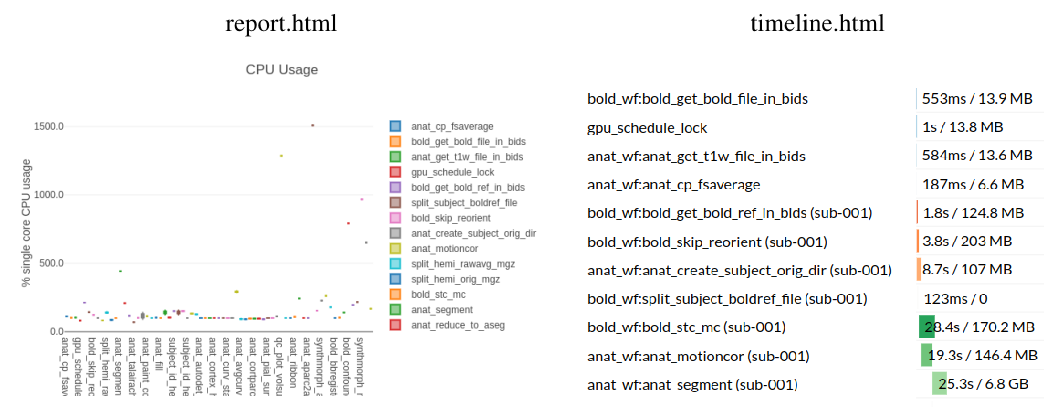
    ├── report.html
    └── timeline.html

DeepPrep automatically generates a descriptive HTML report for each participant and session. View a sample report. The report commences with a concise summary of key imaging parameters extracted from the BIDS meta information. Subsequently, the report provides an overview of the overall CPU and GPU processing times for the data preprocessing. Key processing steps and results for structural images are visually presented, including segmentation, parcellation, spatial normalization, and coregistration. The normalization and coregistration outcomes are demonstrated through dynamic ‘before’ versus ‘after’ animations. Additionally, the report includes a carpet plot, showcasing both the raw and preprocessed fMRI data, along with a temporal signal-to-noise ratio (tSNR) map. Finally, the report concludes with comprehensive boilerplate methods text, offering a clear and consistent description of all preprocessing steps employed, accompanied by appropriate citations. Some examples are shown below:

The visual reports provide several sections per task and run to aid designing a denoising strategy for subsequent analysis. Some of the estimated confounds are plotted with a “carpet” visualization of the BOLD time series. An example is shown below:

Summary statistics are plotted, which may reveal trends or artifacts in the BOLD data. Global signals (GS) were calculated within the whole-brain, and the white-matter (GSWM) and the cerebro-spinal fluid (GSCSF) were calculated with their corresponding masks. The standardized DVARS, framewise-displacement measures (FD), and relative head motion (RHM) were calculated. A carpet plot shows time series for all voxels within the brain mask, including cortical gray matter (Ctx GM), deep (subcortical) gray matter (dGM), white-matter and CSF (WM+CSF), and the rest of the brain (The rest).